


Author: See the Subtle to Understand the Significant
Table of Contents
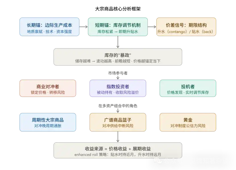
I. Dual Anchor Mechanism for Price Formation
Two: The term structure does not lie
III. The Constraint of Inventory: Cross-Asset Volatility Stratification
Four: Functional Roles of Market Participants
Five: Quantitative Logic of Rollover Yield
Six: The Three-Part Framework for Inflation Hedging
Seven: Considerations for Portfolio Allocation of Commodities
Eight, Summary of Core Methodology
Nine: Introduction to Commodity Portfolio Management
I. Dual Anchor Mechanism for Price Formation
Commodity prices serve two time dimensions simultaneously, and this is the starting point for understanding the entire system.
The long-term anchor is determined by the marginal cost of production—the minimum price at which the highest-cost producer still willing to invest is needed by the market. This anchor moves slowly but has profound implications.
Taking crude oil as an example, in the early 2000s, as spare capacity was exhausted, marginal costs rose significantly, causing the market to shift from the "exploitation phase" (increasing utilization of existing assets) to the "investment phase" (requiring development of entirely new capacity), systematically pushing up the central price level of oil.
In practice, the long-term futures price (typically the 5- to 7-year forward contract) is the best proxy for marginal cost, as producers make price-locking decisions within this time horizon.
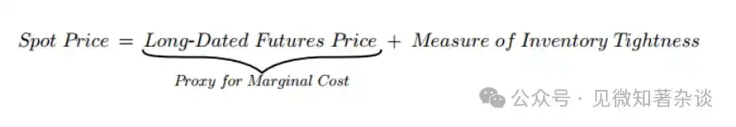
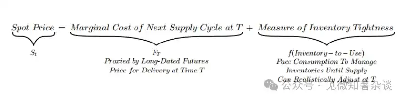
Short-term anchors are dynamically adjusted based on inventory levels. The spread between spot and forward prices (the timespread) is a direct measure of inventory tightness, not a forecast of future price movements.
Methodology: When analyzing any commodity, first separate "how far the forward anchor has moved" from "how much the spot price deviates from the anchor"—the former reflects structural changes on the supply side, while the latter reflects the current physical market tightness.
Two: The term structure does not lie
The term spread has high signal value and is self-enforcing under arbitrage mechanisms:
Contango (backwardation) = Spot price higher than futures price → Market experiences genuine scarcity
Buyers are willing to pay a "spot premium" to receive the asset immediately.
Contango = Spot price lower than futures price → Abundant inventory
Holders prefer to sell spot and buy forward to collect storage costs.
This signal is reliable due to its arbitrage constraint: if a discount is artificially maintained when inventory is abundant, holders will immediately sell the spot and buy the forward to flatten the spread.
Therefore, sustained significant discounts must correspond to genuine physical scarcity.
The extreme case during the COVID-19 period (WTI futures prices falling negative) is the mirror image of extreme contango—inventory filled to the point of having nowhere to store, causing the spot price, after accounting for storage costs, to turn negative.
The role of OPEC deserves separate understanding: the oil-producing alliance can control inventory levels by managing supply, thereby influencing the shape of the curve (maintaining a contango structure indefinitely), but it cannot shift the long-term anchor—high-cost producers (U.S. and Canadian shale oil) determine marginal cost.
III. The Constraint of Inventory: Cross-Asset Volatility Stratification
Storage costs are the underlying explanatory variable for all behavioral differences in commodities, creating predictable cross-commodity stratification:
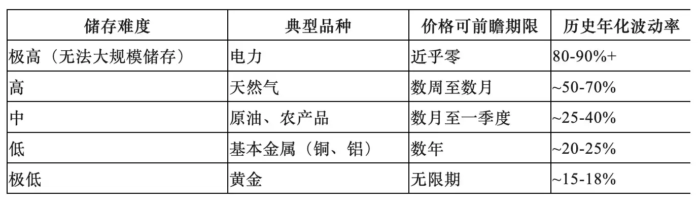
Methodological significance:
Copper is called the "Doctor of Copper" and used as a barometer of the global economy because its low storage cost allows prices to reflect future demand (i.e., expectations of economic growth).
Natural gas and agricultural products are strongly anchored in current physical realities and cannot be explained by "future deficits" as a rationale for current prices—markets for these products absorb premature pricing expectations through inventory accumulation and price declines.
Four: Functional Roles of Market Participants
The three types of participants each have essential economic functions, all of which are indispensable:
1) Commercials: They are the reason the market exists.
Producers lock in prices in advance to transfer price risk by selling in the futures market, creating a structural short position. They are willing to accept a locked-in price below the expected spot price; this discount is the risk premium.
2) Index Investors: Passive liquidity providers.
Buy long-term futures as the counterparty to commercial hedgers, collect the risk premium, make no directional bets, and do not participate in price discovery. Historical data shows no significant correlation between index fund inflows and commodity price movements—they do not drive prices.
3) Speculators: They are the core mechanism for price discovery.
Using the corn market as an example, the USDA’s end-of-season inventory forecast serves as a public benchmark; when the forecast indicates low inventories, speculators buy to push prices higher and slow consumption; when the forecast suggests ample supplies, speculators exit, allowing prices to fall and accelerate consumption.
This real-time adjustment allows markets to smoothly and preemptively reduce or replenish inventories, rather than resorting to violent corrections only after physical shortages have already occurred. The ban on onion futures led to a significant increase in price volatility, serving as a counterproof of speculators' stabilizing role in prices.
Five: Quantitative Logic of Rollover Yield
The excess returns of commodity futures consist of two parts:
Futures excess return = price return + roll yield
Price gains stem from spot price movements, primarily reflected at the front end of the curve (near-term contracts rise sharply due to demand shocks, while longer-term contracts remain relatively stable as they are anchored to marginal cost).
Roll yield comes from the change in contract value as they approach their delivery date:
·Discount market:
As time passes, the contract value increases (as it gets closer daily to the spot price at a premium), generating positive roll yield.
· Premium market:
As time passes, the contract incurs higher storage costs, resulting in negative roll yield (roll decay).
In 2024, Brent crude was an extreme case: the spot price remained virtually flat throughout the year, yet investors achieved double-digit returns solely through roll yield.
Enhanced Roll strategy: Hold nearby contracts under a backwardated curve to maximize roll yield; roll into farther-month contracts under a contangoed curve to reduce roll costs. This is a core active management tool for enhancing long-term returns on commodity futures.
Six: The Three-Part Framework for Inflation Hedging
It is a common mistake to treat "inflation" as a homogeneous whole—three distinct inflation mechanisms correspond to three entirely different hedging tools:
Scenario 1: Late-cycle inflation → Allocate to cyclical commodities
When the economy is overheating, the output gap is positive, demand consistently exceeds supply capacity, and inventories continue to decline. During the late cycle, inventories approach depletion, oil and industrial metals surge sharply, bonds have already weakened, and stock returns begin to plateau—commodities provide ideal diversification at this stage.
The key signal is: inventory has remained consistently below historical seasonal levels, and the rate of depletion is accelerating.
Scenario 2: Supply Shock Inflation → Broad Basket of Goods (Excluding Precious Metals)
Supply shocks (geopolitical events, extreme weather, policy disruptions) have pushed inflation higher while dampening growth, pressuring both bonds and stocks. Commodities, as "interrupted inputs," are often the only assets delivering positive real returns. Due to the unpredictable timing and sources of disruptions, it is essential to hold a broad basket rather than betting on a single commodity.
The reason for excluding precious metals is that, under these circumstances, they may decline inversely due to expectations of interest rate hikes (increasing opportunity cost) and liquidity demands from margin calls.
The Commodity Control Cycle is a structural analytical framework for supply disruption risk, describing a self-reinforcing geopolitical economic logic chain:
Each country turns inward → subsidizes domestic supply → overcapacity drives down global prices → high-cost producers exit → supply becomes concentrated → major players gain both the ability and incentive to weaponize supply → countries further turn inward.
Currently, about 90% of rare earth refining is concentrated in China, indicating a signal of progression into the third/fourth stage of the cycle, meaning the risk of supply disruption has substantially increased.
Scenario 3: Institutional credibility risk → Gold
When the driver of rising inflation expectations is skepticism toward fiscal discipline or central bank independence, or doubt about the neutrality of reserve currencies, gold is the only neutral asset that does not rely on any government's credit.
The classic case of the 1970s (U.S. fiscal expansion + political pressure interfering with monetary policy + Iran’s asset freeze undermining the dollar’s neutrality) clearly illustrates the limits of gold’s role in such scenarios.
Gold is often not an effective hedge in the first two scenarios and may even decline due to expectations of rate hikes and liquidity demands.
Seven: Considerations for Portfolio Allocation of Commodities
1) Fundamental differences from commodity equity
The correlation between commodity equities (mining companies, energy firms) and commodity spot prices is approximately 0.55, while their correlation with large-cap stocks is similarly high at ~0.55. During periods when commodity hedging is most needed—when stocks decline due to inflation and weakening growth—commodity equities often fall alongside the broader market and carry additional company-specific risks (operational disruptions, exposure to cost structures).
Using the 2026 Hormuz incident as an example: the event disrupted approximately 20% of global oil and gas flows, causing significant price increases in commodities; however, producers in the affected regions were unable to capitalize on higher prices due to operational disruptions, while producers in other sectors faced rising energy costs that compressed their profit margins.
2) The "counterintuitive" contribution of volatility
The annualized volatility of BCOM is approximately 15%, higher than U.S. Treasuries (~8%) but lower than U.S. stocks (~19%). Crucially, commodity volatility peaks during periods when both stocks and bonds decline (high inflation + weak growth), meaning that a small allocation to commodities can actually reduce overall portfolio volatility rather than increase it.
Hedging doesn't require a large allocation—transmission of commodity price increases to CPI is far below 100% (doubling oil prices doesn't mean doubling inflation); a small position is sufficient for effective protection.
3) Benchmark Selection and Regional Adaptation
·S&P GSCI: Production-weighted, energy makes up ~52%, volatility around 20%
·BCOM: More balanced, with energy, metals, and agricultural products each at approximately 29%, 35%, and 36%, respectively, and a volatility of about 15%, making it the current mainstream investment benchmark.
Important note: Both benchmarks use U.S. natural gas (Henry Hub) to represent natural gas exposure; for European investors, replace with TTF, and for Asian investors, replace with JKM, otherwise local energy inflation will be systematically under-hedged.
Eight, Summary of Core Methodology
1. Pricing Analysis: Always distinguish between the "forward anchor (marginal cost)" and the "term spread (inventory)" dimensions, using long-term futures to proxy the former and the 1M-13M spread to proxy the latter.
2. Product Selection: Using storage economics as the axis, distinguish between energy and agricultural products that are "present-focused" and metals that are "forward-looking," each corresponding to different analytical frameworks and holding instruments.
3. Inflation Hedge: Clearly distinguish among three inflation mechanisms and reject oversimplified "basket inflation" judgments.
4. Return Attribution: When holding commodity futures, separate price returns from roll returns; the latter, driven by the curve shape, can be actively managed through an enhanced roll strategy.
5. Risk signal: Monitor the stage of the commodity control cycle—when global supply concentration continues to rise (a third-stage signal), the structural value of hedging against supply disruption risk increases.
Commodity Introduction Guide for Portfolio Managers
Zero, Executive Summary
This beginner's guide provides a practical introduction to commodity markets—how they work, when to protect your portfolio, and how to gain exposure.
Seize the present, invest in the future. Commodity prices operate across two time dimensions: on one hand, they are anchored by the marginal cost of future production (determined by geology, technology, and capital intensity) to incentivize new supply; on the other, they regulate current consumption to manage inventories. When inventories are low, prices rise to dampen demand and prevent depletion; when inventories are ample, prices fall to accelerate consumption and reduce excess stock.
The constraint of inventory. Inventory resolves the inherent time mismatch in commodity markets, where supply decisions are made months or even years before consumption occurs. But storage is not free. The harder a commodity is to store, the stronger the constraint storage costs impose on prices—shaping price volatility, limiting the forward-looking capacity of commodity markets, and pulling prices back toward current physical realities.
Not all inflation is the same. Three different inflation shocks require different hedging tools.
1) Late cycle: Hedge with cyclical commodities. When the economy overheats and demand exceeds production capacity, inflationary pressures build as inventories continue to be drawn down. During the late cycle, as inventories approach depletion, cyclical commodities such as oil and industrial metals tend to rise—just as bond prices weaken and stock returns begin to soften.
2) Supply disruptions: Hedge with a broad commodity basket (e.g., including precious metals). When supply disruptions occur (such as Russia cutting off about 40% of Europe’s natural gas supply in 2022), inflation rises while growth slows, dragging down bond and stock prices. At such times, commodities—acting as the disrupted inputs—are among the few assets that can deliver positive real returns. Since the source and timing of disruptions are inherently unpredictable, a broad commodity basket (e.g., including precious metals) offers the most robust protection.
3) Institutional credibility risk: Hedge with gold. When concerns about institutional trust and macroeconomic policies drive up inflation expectations, gold serves as a key neutral asset whose value does not rely on any government backing.
Achieve portfolio stability through commodity volatility. Commodities are volatile, but their prices often surge when stocks and bonds decline simultaneously—such as during periods of high inflation and weak growth—so a small allocation to commodities can reduce overall portfolio volatility rather than increase it.
Gain exposure. Traditional benchmarks like BCOM serve as a practical starting point. Investors seeking more customized hedges can consider region-specific exposure (since U.S. benchmarks may not adequately hedge energy inflation in Europe or Asia), tilt toward their most concerning inflation mechanisms, and adopt enhanced roll strategies to improve returns from long-term commodity futures holdings.
How do products work?
1.1. Seize the moment, invest in the future
The harvest season for U.S. corn lasts only a few weeks in the fall, but the crop produced during this brief window must meet the needs of the United States—and the world—for the next twelve months. To achieve this, prices must perform a balancing act: high enough to prevent depletion before the next harvest, yet low enough to avoid excessive stockpiles by year-end. The right price adjusts consumption—slowing it down or speeding it up—to deplete inventories at just the right rate (Chart 1).
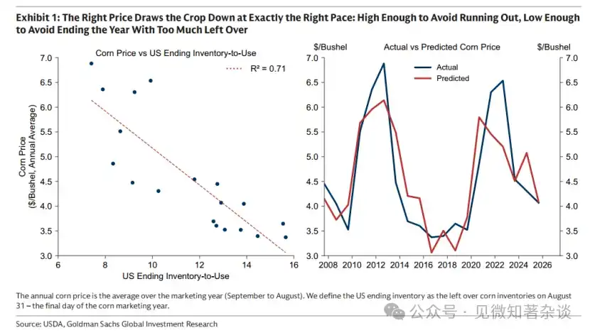
Chart 1: The correct price consumes crops at just the right rate: high enough to avoid depletion, low enough to prevent excess surplus at year-end.
But price has another task: ensuring planting for the next harvest. If the marginal cost of future production rises—due to soaring fertilizer prices, declining yields, or scarcer high-quality farmland—the price anchor will also rise, and prices will adjust accordingly, consuming inventories around this higher level.
The corn market operates on two temporal dimensions: prices are anchored by the marginal cost of future production (dependent on geology, technology, and capital intensity), while ensuring that current available inventories are consumed at an appropriate rate.

This logic applies to all commodity markets, whether production is seasonal (such as agriculture) or continuous (such as oil and copper)—for the latter, the rate at which supply is released to the market is largely locked in by decisions made several quarters or even years before consumption occurs.
1.2. Anchored to Forward
We can use long-term futures to approximate changes in marginal cost. Producers make capital investments and production decisions far in advance, locking in prices by selling futures years ahead to manage price risk. Projects proceed only when the locked-in price covers costs, making long-term futures prices a practical proxy for marginal cost—the lowest price at which the highest-cost, last-needed producer is still willing to invest.
As shown in Figure 2, marginal costs change slowly but can shift significantly over time. In the oil market, marginal costs rose sharply after the mid-2000s, as spare capacity—primarily built in the 1970s—was exhausted in the early 21st century. This transition pushed the market from the exploitation phase, where supply growth came from increased utilization of existing assets at low cost, into the investment phase, requiring the construction of new, next-generation capacity at significantly higher costs.
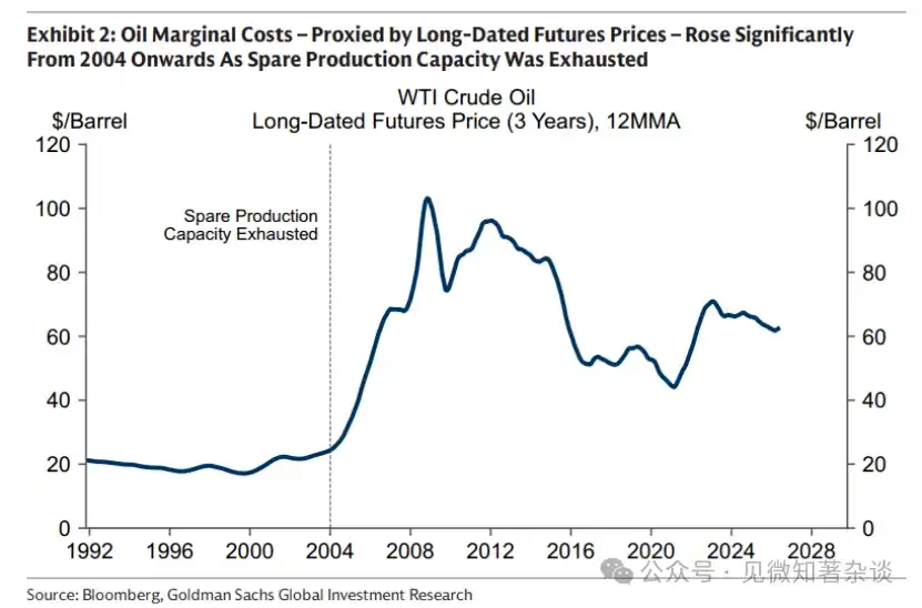
Chart 2: Oil marginal cost, proxied by long-term futures prices, has risen significantly since 2004 as spare capacity has been exhausted.
1.3. The term spread doesn't lie
Since long-term futures reflect the marginal cost of future supply, spot prices are anchored around long-term futures prices.
Any deviation between the spot price and the long-term futures price—defined as the term spread—exists solely to manage inventory and thus directly reflects current physical conditions.

· Scarcity imparts value to near-term deliveries. Buyers pay a premium for immediate delivery to secure immediate access to the commodity, pushing spot prices above futures prices. This resulting downward-sloping curve—spot premium—merely reflects that contracts closer to delivery are more valuable than distant ones when inventories are tight, not that prices are expected to fall (red section in Chart 3).
· Adequate inventory eliminates the need to pay a premium for immediate delivery. Choosing to wait for delivery requires holding inventory during the period—which can be a significant cost when inventory levels are high. As a result, the spot price trades below the futures price, creating an upward-sloping curve—known as contango—that reflects the storage costs embedded in forward contracts, rather than an expectation of rising prices (blue section in Chart 3).
The COVID-19 pandemic pushed the futures premium for oil to extremes. As the economy stalled, demand for oil collapsed and storage facilities became completely full. With nowhere to store it, the spot price of oil fell into negative territory.
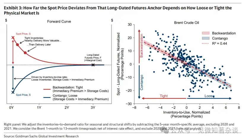
Chart 3: The extent to which the spot price deviates from the long-term futures anchor depends on the looseness or tightness of the physical market.
These term spreads don't lie. The spot price cannot sustainably trade above the futures price (contango) without genuine scarcity.
The reason is that if the spot price is maintained above the futures price despite ample inventory and no genuine need to pay a premium for immediate delivery, inventory holders who do not need to use the commodity immediately can sell at the higher spot price and repurchase at a lower price in the forward market for future delivery, thereby avoiding storage costs during the period.
As more holders take the same action, spot selling pressure increases, pulling the spot price lower relative to futures and quickly returning the market to a futures premium state.
OPEC can shape the curve, but cannot move the anchor.
Although term spreads cannot lie about physical reality, large enough participants—such as producer groups—can influence the physical reality itself. This is why oil is typically traded in a contango state: by managing supply, OPEC can control the inventory levels reflected in the term spread, thereby influencing the shape of the curve.
By deliberately withholding oil and maintaining spare capacity, OPEC can stabilize inventories during shortages—releasing supply when prices surge to dampen volatility. Lower volatility, in turn, reduces the incentive to substitute for oil, supporting long-term oil demand. This supply management keeps inventories tight and the curve in contango, enabling OPEC to sell at spot prices higher than those of its peers (who hedge at lower futures prices) and generate larger price movements with relatively modest production adjustments.
While OPEC can shape the curve, it cannot move the anchor. Long-term prices are set by marginal high-cost producers—and that is not OPEC. High-cost production from the U.S. and Canada sets the anchor: the minimum price at which it’s worthwhile to produce the next barrel of oil. OPEC simply does not have enough spare capacity to replace all of this high-cost supply.
1.4. The Constraint of Inventory
Inventory bridges the inherent time mismatch in commodity markets, where supply decisions are made months or even years before consumption occurs. But holding inventory comes at a cost, and that cost matters. The harder a commodity is to store, the stronger the storage cost constrains its price. These storage constraints shape how commodity markets behave—how volatile prices are, how far ahead markets can look, and how quickly prices are pulled back toward current physical realities. The economics of storage is the inescapable constraint on commodities.
1.5. Easy to store, lower volatility
Inventory dampens volatility by allowing markets to gradually absorb shocks. Without this buffer, prices must react immediately, leading to larger fluctuations—similar to electricity markets, where large-scale storage is challenging and supply and demand must be matched second by second. Natural gas storage is costly and difficult, leaving only a small buffer to absorb unexpected changes in demand, resulting in very high volatility. In contrast, metals are easy to store and readily buffer—hence, their volatility is much lower (Chart 4).
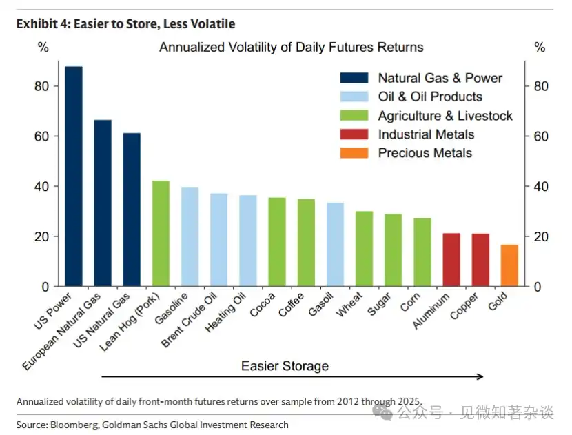
Chart 4: Easy to store, lower volatility
1.6. Unlike bonds and stocks, commodities cannot be forecast far into the future.
Expected shortages are typically not priced into commodity prices, as inventory constraints continuously pull prices back to current physical realities. If prices rise prematurely due to expectations of future shortages, consumption slows and supply increases, leading to inventory accumulation. Thus, long-term shortages can cause near-term surpluses. With nowhere to go for excess inventory, rising storage costs force prices down—often well before the expected shortage materializes.
This is particularly evident in energy and agriculture, where supply can respond quickly to price increases and high storage costs lead to rapid inventory accumulation and swift price corrections. This is less pronounced in metals: because supply adjustments are slow and storage costs are low, inventory buildup is typically controlled rather than disruptive, allowing metal prices to look further ahead without immediate price corrections (Chart 5).
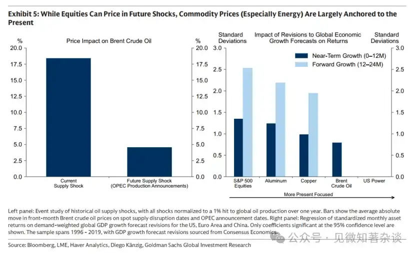
Chart 5: While stocks can price in future shocks, commodity prices—especially energy—are primarily anchored to the present.
1.7. Who trades commodities, and why?
Three distinct participant groups—commercial institutions, index investors, and speculators—actively participate in commodity markets, each helping to bridge the time gap between supply decisions and consumption (Chart 6).
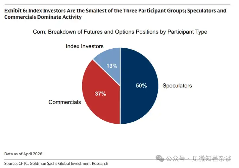
Chart 6: Index investors are the smallest of the three participant groups; speculators and commercial institutions dominate activity.
· Commercial institutions—the reason markets exist—are primarily producers. Producers invest capital and plan production well in advance, but prices may fluctuate significantly before the first barrel of oil is shipped. To hedge against this price risk, producers sell futures contracts, typically at a price below the expected spot price. This discount is the risk premium: the cost of transferring price risk to others.
· Index investors—passive liquidity providers—are the fixed buyers on the other side of long-term futures sales, in exchange for a risk premium. They hold no directional view on price and simply go long on commodities as an asset class, mechanically rolling their positions over time. As a result, they do not drive price movements (Chart 7).
· Speculators—price discoverers—bring new information into prices and help regulate the rate of inventory consumption in real time. In the corn market, the link between forward fundamental expectations and speculative buying is particularly clear, as the U.S. Department of Agriculture releases forward-looking estimates of ending inventory, providing a public benchmark for expected supply and demand balances.
As shown in the left chart of Figure 8, the lower USDA inventory forecast coincided with large speculative long positions. Speculators buy when they expect inventories to be depleted before the end of the season, driving up prices and slowing consumption; they exit when they anticipate excess inventory at year-end.
By converting inventory expectations into prices in real time, speculators enable the market to adjust in advance and smoothly (right chart, Figure 8). Without them, prices would only adjust once the shortage had already occurred—leading to more sudden and disruptive corrections.
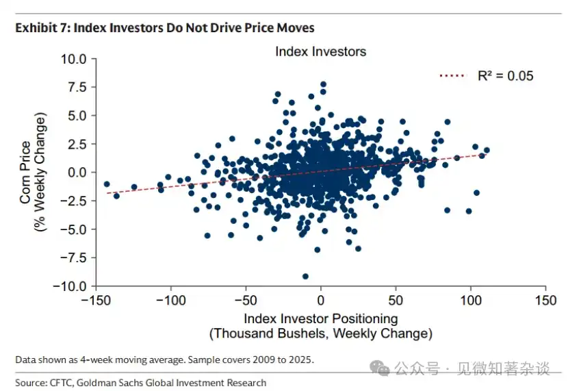
Chart 7: Index investors do not drive price movements
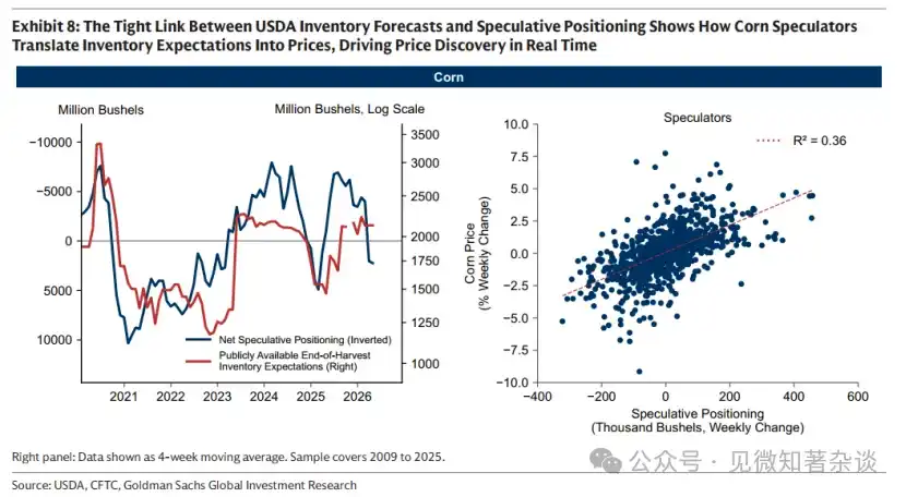
Chart 8: The close correlation between USDA inventory forecasts and speculative positions shows how corn speculators translate inventory expectations into price, driving price discovery in real time.
Case: The Onion Futures Ban Backfired
Sometimes, speculators come under scrutiny for their role in commodity markets. However, a market without speculators often experiences greater volatility, not less—as the famous example of the onion market illustrates.
In 1955, Vincent Kosuga, a futures trader raised as an onion farmer, and his partner Sam Siegel manipulated the onion market at the Chicago Board of Trade. By autumn, they controlled over 99% of the onions in Chicago, amassing approximately 14,000 metric tons (30 million pounds). Onions were shipped from across the country to Chicago, filling warehouses to capacity and driving up storage costs.
Under pressure from rising storage costs, they changed their strategy—threatening to flood the market unless onion growers bought back their inventory. When the onion growers intervened, the pair established massive short positions in onion futures. By the end of the harvest season in March 1956, they still flooded the market, causing prices to plummet from $2.75 per bag to just 10 cents—below the cost of the bags themselves.
KuCoin and Siegel made millions from their short positions. Many farmers went bankrupt. This event led the U.S. Congress to pass the Onion Futures Act in 1958, completely banning onion futures trading. To this day, people can trade futures on oil, wheat, copper, and even frozen orange juice—but not onions.
But the ban had the opposite effect. Without speculators to bring information into prices and adjust inventory consumption in real time, onion prices became more volatile—not less (Chart 9).
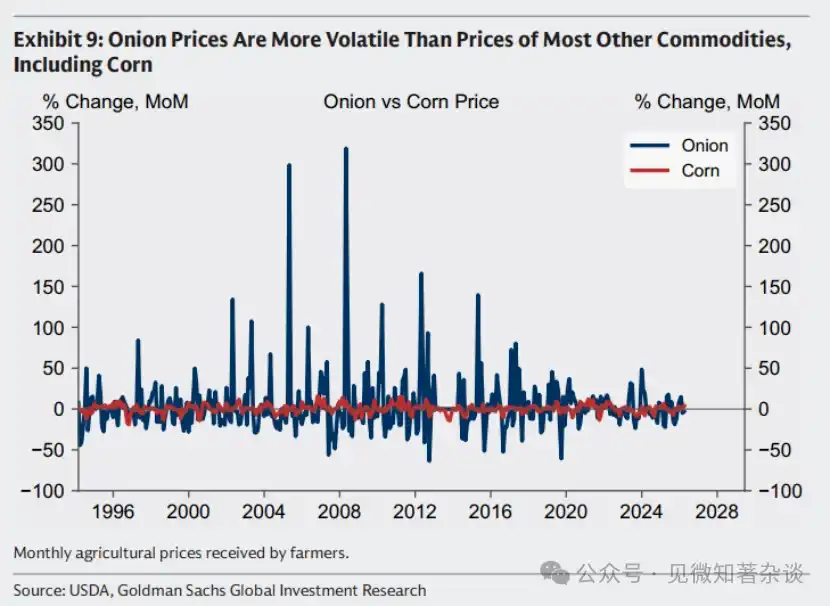
Chart 9: The price of onions is more volatile than most other commodities, including corn.
1.8. The Role of Roll Yield in Commodity Returns
The return on commodity futures (above the interest rate) consists of two components: price return and roll yield. We illustrate the role of roll yield with a simple assumption.
Price return. Increased demand has strained inventory and pushed spot prices up by $20. As shown in Chart 10, this $20 increase is concentrated at the front of the curve, while the back end remains anchored to marginal cost.
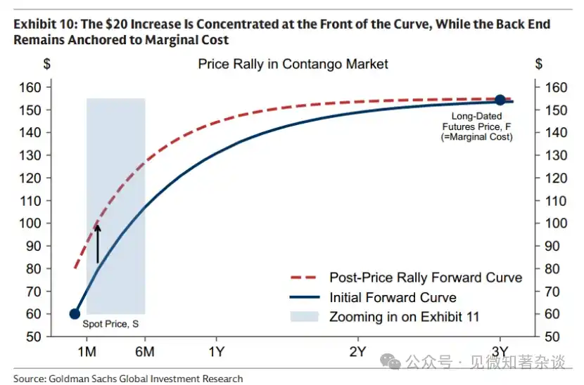
Chart 10: The $20 increase is concentrated at the front of the curve, while the back remains anchored at marginal cost.
Roll yield. A commodity futures contract is essentially a claim to physical delivery in the future—such as in August 2026. As time passes, the contract grows closer to physical delivery. Therefore, even if the spot price itself remains unchanged, its value may rise or fall due to the shape of the futures curve.
· In a futures market with ample supply and a premium, holding a contract may incur costs over time. Even if the spot price remains unchanged, the same August 2026 contract may depreciate over time, as each passing week includes storage costs. When inventory is abundant, these storage costs can be substantial.
In the hypothetical example in Chart 11, simply moving one month closer to the delivery date results in a $12 loss, as storage costs fully offset any immediate delivery premium. This leaves only $8 of the original $20 spot price increase. One way to reduce this drag is to hold contracts further out on the curve, where the slope is flatter—for example, at the six-month point, the same time progression might incur only a $1 cost.
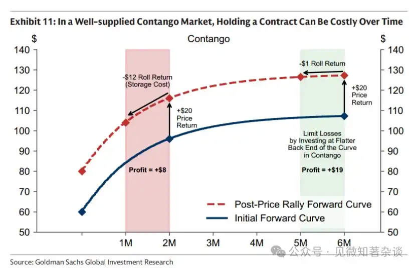
Chart 11: In a futures market with ample supply and premium, holding a contract may incur costs over time
· In a scarce, contango market, time is on your side. Each day closer to delivery, the value of a claim to a good that is currently difficult to obtain increases, even if the spot price remains unchanged (Chart 12).
The power of roll yield can be significant. In 2024, the spot price of Brent crude oil started at $75.89 per barrel and ended at $75.93—nearly unchanged—yet investors achieved double-digit returns solely from roll yield.
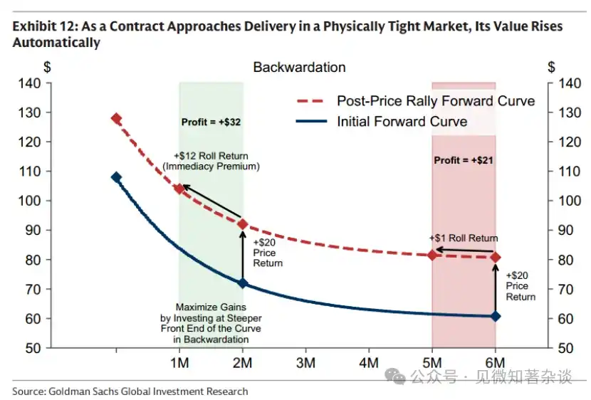
Chart 12: When a contract approaches delivery in a market with physical tightness, its value automatically increases.
Therefore, most index investors adopt an enhanced rollover strategy: investing closer to the front of the curve when the spot is at a premium to maximize rollover returns, and extending further out when the futures are at a premium to minimize rollover costs.
II. The Role of Commodities in a Diversified Portfolio
2.1. Not all inflation is the same — different inflation shocks require different hedging tools
Some investors view commodities and gold as a single inflation hedge. In reality, inflation typically arises through three distinct mechanisms—late-cycle inflation, supply disruptions, and institutional credibility risk—each requiring a different hedging tool.
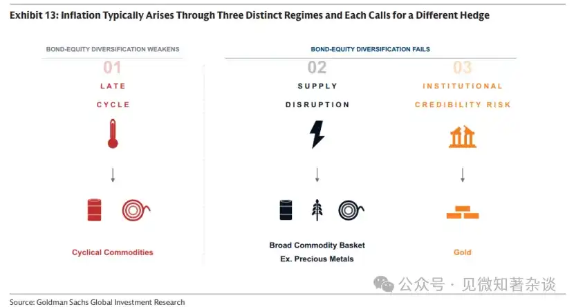
Chart 13: Inflation is typically generated through three distinct mechanisms, each requiring different hedging tools
Mechanism 1: Late Cycle — Hedge with Cyclical Commodities
When the economic cycle overheats, equities initially benefit from strong growth. But as the economy begins to exceed its productive capacity (economists call this a positive output gap), inflationary pressures build and real bond returns weaken. Over time, rising input costs compress profit margins, and equity growth begins to stall. It is precisely at this stage—when bond prices weaken and equity returns start to lose momentum—that commodities often provide diversification through stronger returns.
Commodities typically perform well in the late stage of the cycle, as a positive output gap indicates demand exceeding supply. In commodity markets, this imbalance manifests as sustained inventory drawdowns. By the late stage of the cycle, inventories have been depleted for an extended period and are nearing exhaustion, pushing prices higher—particularly for cyclical commodities such as oil and industrial metals.
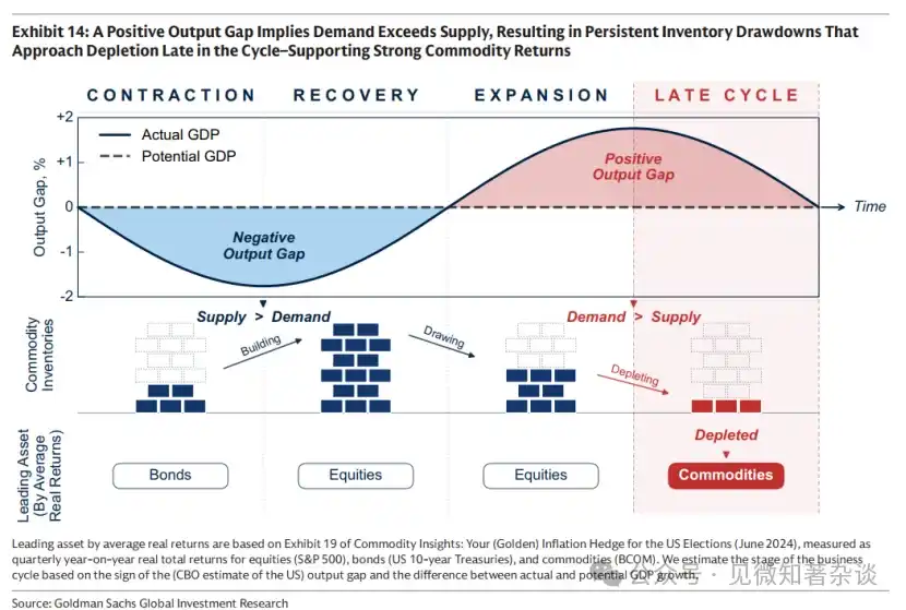
Chart 14: A positive output gap indicates that demand exceeds supply, leading to sustained inventory depletion nearing exhaustion in the later stage of the cycle—supporting strong commodity returns
The return of the old economy
The late cycle is the moment when an expansionary economy encounters its physical constraints—what our team calls "the return of the old economy."
During prolonged phases of ample supply, commodity returns are typically weak, with capital flowing toward the dominant growth themes of the time, such as the internet boom of the late 1990s. Over time, underinvestment in new commodity supply combined with sustained demand growth erodes excess capacity, inventories begin to deplete, and growing economies become increasingly exposed to physical constraints.
At that moment, the market transitioned from the extraction phase—where demand growth was met by increasing utilization of existing capacity—to the investment phase. In the investment phase, long-term commodity prices must rise structurally, as easily accessible reserves are depleted, idle capacity is exhausted, and every additional barrel or ton now requires new capital to produce.
Uncertainty may cause the underinvestment cycle to persist. When investors fear that cheap supply could reemerge once new projects come online, capital tends to remain on the sidelines—whether due to policy support (such as tariffs or price floors) that could reverse restrictions on low-cost foreign supply, or because current geopolitical disruptions constraining supply may eventually be resolved. Paradoxically, the very uncertainty that pushes prices higher in the short term may delay the investment needed to bring prices back down in the medium term.
Mechanism 2: Supply disruption—hedge with a broad commodity basket (e.g., including precious metals)
When supply disruptions occur (such as Russia cutting off about 40% of Europe’s natural gas supply in 2022), inflation rises while growth slows, simultaneously dragging down bond and stock prices. In such scenarios, commodities—acting as the disrupted inputs—are among the few assets capable of delivering positive real returns. Because the source and timing of disruptions are inherently unpredictable, a broad commodity basket (e.g., including precious metals) offers the most robust protection.
Product control cycle
Although the exact timing of disruptions cannot be predicted, the risk of disruption tends to rise structurally as global economic integration declines. This unfolds through a self-reinforcing cycle that requires no malicious actors—each step is a rational response to the previous one (Chart 15).
As countries turn inward, governments are implementing measures to insulate supply chains through tariffs, subsidies, and state-supported investments, aiming to replace imports wherever possible and stockpile when replacement is not feasible.
These incentives to stimulate supply may lead to supply exceeding domestic demand. The resulting surplus is exported, putting downward pressure on global prices.
Lower prices force high-cost producers elsewhere to exit the market, ultimately concentrating supply among fewer participants.
· When supply becomes concentrated in fewer hands, dominant producers can use it as a geopolitical and economic lever—increasing the risk of disruptions, commodity price volatility, and inflationary pressures. This, in turn, prompts other countries to further isolate their supply chains, reinforcing the cycle.
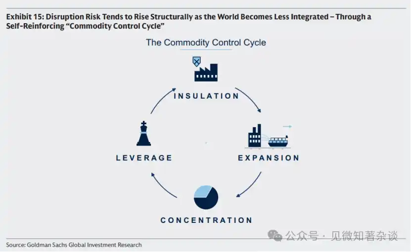
Chart 15: As the world becomes increasingly fragmented, disruption risks often rise structurally—through a self-reinforcing "commodity control cycle"
Investors seeking to hedge against portfolio disruption risks may consider acting when commodity control cycles are nearing or have reached Step 3—when countries turn inward and supply becomes increasingly concentrated in regions with higher geopolitical or trade dispute risks (Chart 16). At that stage, Step 4 becomes a genuine risk: supply comes under the control of a few actors with both the capability and potential incentive to use it as an economic or geopolitical lever.
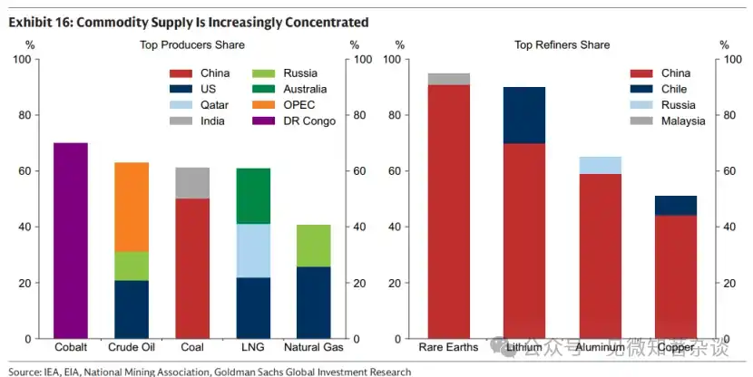
Chart 16: Increasing Concentration of Commodity Supply
Mechanism 3: Institutional Reputation Risk — Hedging with Gold
In the first two inflation scenarios—late-cycle inflation and supply disruptions—gold is not an effective hedge. Instead, gold typically declines initially: higher inflation may lead markets to anticipate rate hikes, increasing the opportunity cost of holding non-yielding assets, and stock market declines may trigger margin calls and liquidations of gold due to its high liquidity and ready availability as a source of cash.
Gold serves as a narrow hedge against inflation: when inflation expectations rise due to concerns about institutional credibility or macroeconomic policy, leading to simultaneous sell-offs in bonds and stocks, gold emerges as a key neutral asset whose value does not rely on any government backing.
The 1970s serve as a classic case. Massive U.S. fiscal expansion and political pressure on the Federal Reserve to lower interest rates led to runaway inflation, while the freezing of Iran’s central bank assets raised doubts about the geopolitical neutrality of the dollar. As investors sought value outside the financial system—namely, an asset that could neither be devalued nor frozen—the price of gold surged.
2.2. Provide diversification during critical periods
As shown in Chart 17, during every 12-month period when both stock and bond real returns were negative, commodities or gold generated positive real returns. The "golden age" of the 60/40 portfolio from the late 1990s to 2022 coincided with highly globalized supply chains and strong institutional trust, enabling Mechanism 2 (supply disruptions) and
Mechanism 3 (Institutional Credibility Risk)—these two inflationary mechanisms most destructive to traditional portfolios—are largely absent. When supply chains become fragmented and/or concerns about institutional credibility and macroeconomic policy rise, the rationale for allocating to commodities and/or gold reemerges.
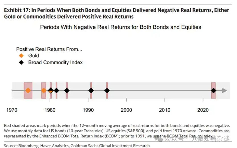
Chart 17: During periods when both bond and stock real returns were negative, gold or commodities generated positive real returns.
Although positive stock returns can still offset negative bond returns in the late stage of the cycle, the upward momentum of stocks begins to weaken, and the correlation between stocks and bonds turns positive, reducing diversification benefits. In this stage, commodities can provide additional diversification, as they often perform strongly during the late phase of the cycle.
2.3. Commodity-linked stocks cannot replace physical commodities
Some investors seek commodity exposure through equities in commodity-producing sectors (miners, energy producers, and agricultural companies) to gain leveraged upside potential. Profits, reserves, and cost discipline can amplify returns relative to movements in the underlying commodity prices.
However, this amplification effect is two-sided—and often has adverse effects when investors most need commodity exposure. Commodity stocks are still equities at their core and exhibit strong correlation with the broader market (~0.55). In the late stage of the cycle, as inventories near depletion, commodity prices may surge sharply, while producer stocks, priced based on forward cash flows, may weaken alongside the broader market due to slowing growth or rising risks of interest rate hikes.
Unlike direct commodity exposure, stock investors also bear company-specific risks: operational disruptions, management decisions, balance sheet pressures, and input cost risks. These risks are most pronounced during supply disruptions. When supply shocks occur, commodity prices often rise in tandem—such as during the 2026 Hormuz incident, which disrupted approximately 20% of global oil and gas flows and critical chemical inputs, affecting agriculture and metals.
Rising commodity prices do not necessarily translate into strong performance for related stocks. If producers of the affected commodities suffer operational setbacks, they may not benefit from higher prices. Meanwhile, producers in other commodity sectors, even as their own commodity prices rise, may face compressed profit margins—since energy is a critical input for mining, smelting, and agriculture.
2.4. Achieving Portfolio Stability Through Commodity Volatility
Commodities are volatile: BCOM has an annualized volatility of approximately 15%, higher than U.S. fixed income’s ~8% but lower than U.S. stocks’ ~19%. However, commodities typically experience their largest gains during periods of high inflation and weak growth, which simultaneously weigh on stock and bond prices.
Therefore, commodity allocation may reduce the overall portfolio volatility rather than increase it. As shown in Chart 18, adding commodities to a stock-bond portfolio may allow investors to take on lower risk for the same expected return, or achieve higher returns at the same risk level.
Commodities do not require a large allocation to serve as an effective hedging tool. As inputs, commodity price increases are only partially passed through to consumer prices—a doubling of oil prices does not mean a 100% rise in inflation. Therefore, even a small allocation to commodities can have a significant impact and, under normal conditions, can fulfill its role during periods of equity-bond diversification failure without consuming a large portion of the portfolio’s risk budget.
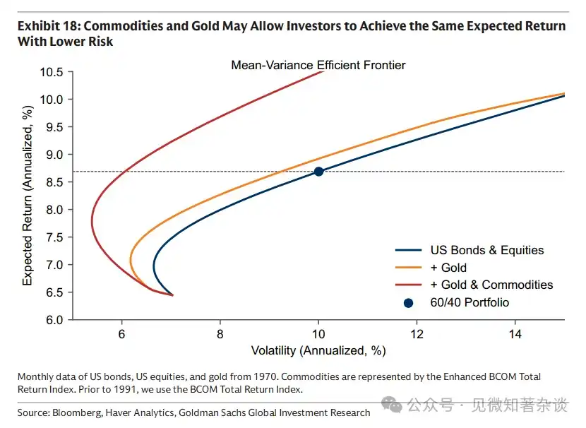
Chart 18: Commodities and gold may enable investors to take on lower risk for the same expected return.
III. Considerations for Building a Product Basket
3.1. Traditional Benchmarks
Two standard commodity benchmarks are the S&P GSCI and the BCOM. The S&P GSCI is production-weighted—designed to approximate the global consumption basket—resulting in a large weight on energy. The BCOM is the more widely used benchmark among investors today, with a more balanced allocation across energy, metals, and agriculture, resulting in typically lower volatility than the S&P GSCI (20% versus 15% for BCOM).
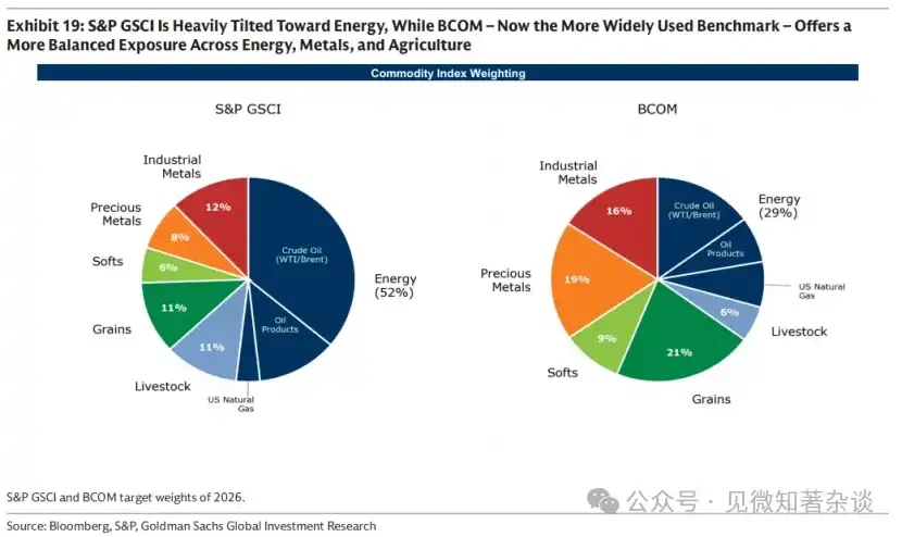
Chart 19: The S&P GSCI is heavily weighted toward energy, while the BCOM (currently the broader benchmark) provides a more balanced exposure across energy, metals, and agriculture.
3.2. Geographical Factors
Standard commodity benchmarks are often U.S.-centric, and thus may be slightly under-hedged in addressing energy and food inflation relevant to non-U.S. investors. For example, natural gas is a regional market: European investors are better off hedging with European TTF, and Asian investors with JKM, rather than using the U.S. Henry Hub natural gas contracts included in the BCOM and S&P GSCI.
3.3. Tilt toward the target inflation mechanism
Investors seeking to hedge against specific inflation mechanisms may wish to adjust their commodity baskets accordingly. As summarized in Chart 20, cyclical commodities hedge against late-cycle inflation, broad commodity baskets (e.g., including precious metals) hedge against supply disruption risks, and gold hedges against inflation only when concerns stem from market doubts about institutional credibility or macroeconomic policy.
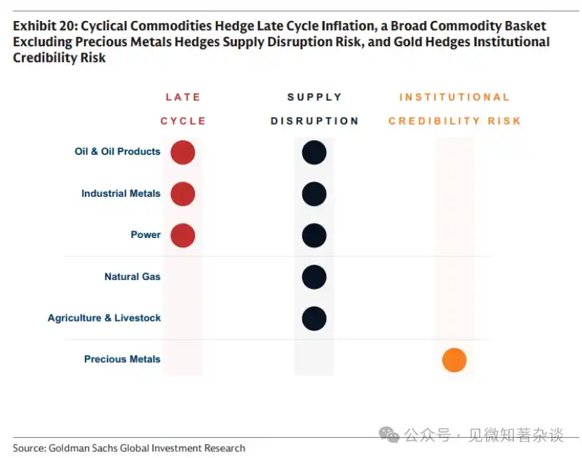
Chart 20: Cyclical commodities hedge against late-cycle inflation, broad commodity baskets (e.g., including precious metals) hedge against supply disruption risks, and gold hedges against institutional credibility risks.
The effectiveness of a commodity as a hedge against supply-driven inflation depends on two factors: its direct or indirect weight in the inflation basket, and the share of supply that could be disrupted. Energy scores highly on the first factor, both historically and currently. Industrial metals and rare earths have lower inflation weights, although their importance has been rising due to increased demand for grid infrastructure from global electrification and the shift toward renewable energy sources. However, on the second factor, industrial metals and rare earths stand out—refining is highly concentrated, with China controlling approximately 90% of global rare earth processing (Chart 16). Such large-scale disruptions, even if they only indirectly affect consumer prices (e.g., as inputs for automobiles), could generate significant spillover effects.
3.4. USD and Commodities
Products are priced in U.S. dollars, which is important for non-U.S. dollar investors, but the relationship between the U.S. dollar and commodities varies by industry.
In the energy sector, causality typically flows from commodity markets to currency markets. Energy is a significant component of the current account; given that the United States is now a major energy exporter while most economies remain importers, higher energy prices can support the dollar against other currencies.
In metals and agriculture, this relationship is often inverse—flowing from currency to commodities—because supply or cost structures are primarily set by local currencies. Cyclical forces may also simultaneously drive both commodity and currency markets. Industrial metals are especially sensitive to U.S. monetary policy and global growth expectations: lowering policy rates weakens the dollar and often boosts demand for metals. As a result, copper often serves as a liquidity proxy for global growth—and the renminbi exchange rate—reflecting China’s dominant share of global copper consumption (58%).
3.5. Enhanced Rollover Strategy
As described in Section 1.8, commodity index returns consist of two components: spot price return and roll yield—the gain or cost arising simply from holding a commodity futures contract as it moves closer to delivery over time. In a market with futures premium, storage costs exceed any immediate delivery premium, making this time passage a cost. In a market with spot premium, physical tightness pulls spot prices above futures, making the same time passage a gain.
Most index investors use an enhanced rollover strategy to manage returns from holding commodities over time: automatically investing in the front of the curve to capture roll yield when the market is in contango, and extending further along the curve to minimize roll costs when the market is in backwardation.
Appendix: A Simple Framework for Product Pricing
The spot price adjusts the rate of inventory consumption around the long-term anchor.
In Section 1.1, we showed that the spot price consists of two components: a slowly moving anchor set by the marginal cost of future supply, and a fast-adjusting term that regulates current inventory.
This decomposition implies that the term spread—the deviation between the spot price and the long-term futures price—corresponds exactly to the inventory tightness measure: term spread = spot price - long-term futures price = inventory tightness measure
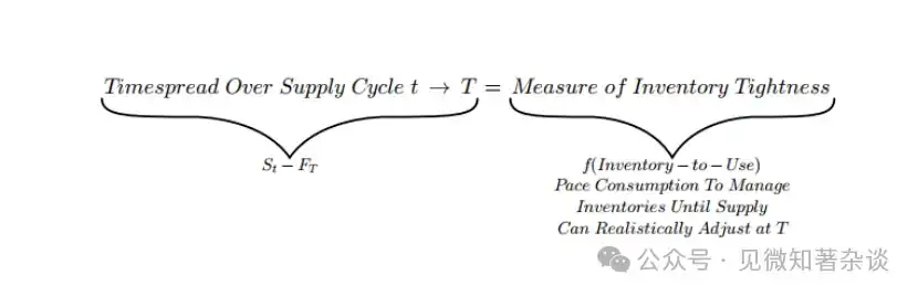
The term spread moves with the degree of inventory tightness—reflecting whether the market is paying a premium for immediacy or bearing storage costs.
Therefore, the term spread directly reflects the current physical tightness, as measured by the inventory utilization ratio. Depending on the level of tightness, the market either pays a premium for immediacy or incurs storage costs (Chart 21).
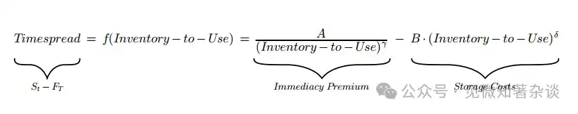
· Scarce physical supply (low inventory-to-use ratio) makes immediate delivery valuable. The immediacy premium dominates, pushing spot prices above futures prices—resulting in a downward-sloping curve and a positive roll yield (contango).
· Adequate inventory (high inventory-to-use ratio) eliminates the need to pay a premium for immediate delivery. Choosing to wait for delivery requires holding inventory during the period—which can be a significant cost when inventories are high. Storage costs dominate, pushing spot prices below futures prices—resulting in an upward-sloping curve and a negative basis (futures premium).
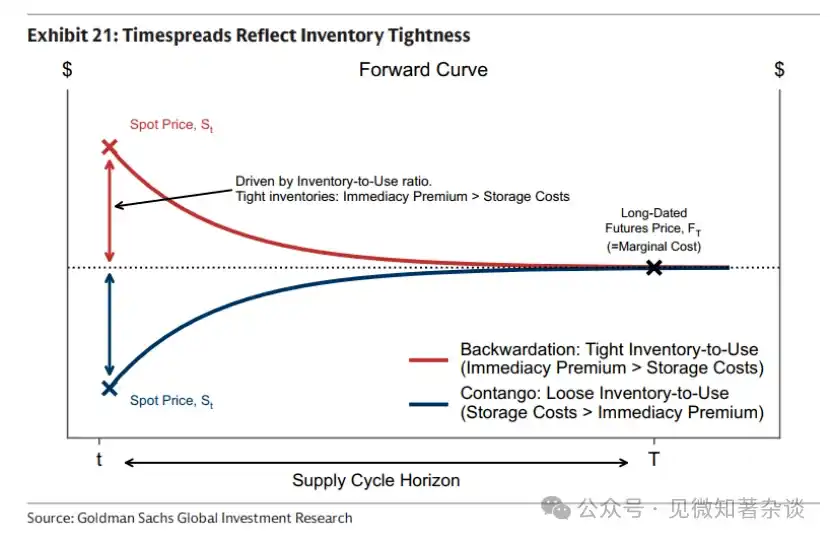
Chart 21: The term spread reflects inventory tightness
Why do forward curves vary across different commodities?
Two elasticities determine how strongly the term spread responds to inventory tightness:
·γ: The steepness with which the immediacy premium rises as inventory decreases.
·δ: The rate at which storage costs increase as inventory rises.
These elasticities vary by commodity. In the energy sector, γ and δ are often both high, as depleting inventories can cause disruptive economic impacts and storage costs are high. In the metals sector, these elasticities tend to be lower, as the consequences of shortages are less severe and storage costs are relatively low.
Why commodities, especially energy, cannot be forecast far into the future
Our framework explains why commodities, especially energy, are primarily spot assets and cannot sustainably price above their supply adjustment cycle fundamentals.
To understand why, consider this scenario: the market attempts to determine inventory levels for a time horizon beyond T (i.e., the point at which supply can respond). For example, suppose the market tries to price in a future positive demand shock by pushing up the current spot price.
This implicitly requires more inventory coverage than under reasonable adjustment speeds. As a result, the inventory coverage ratio rises above its reasonably adjusted level. The market moves from the correct adjustment point (blue) to an over-adjusted point (red), along the curve connecting the term spread to the inventory usage ratio (Charts 22 and 23).
As inventory accumulates, the rate at which the spot price is forced down depends on δ, the elasticity of storage costs.
· Energy: High δ, short T. As inventory accumulates, storage costs rise rapidly. High spot prices dampen demand and encourage a relatively swift supply response, leading to inventory buildup and increased storage pressure. Compared to the forward anchor FT, the spot price declines sharply (in Chart 22, the red overbought points show S_t deviating significantly from F_T). High storage costs thus enforce discipline—inventory cannot be planned for durations exceeding T without incurring substantial price penalties.
· Metals: δ is low, T is long. As inventory accumulates, storage costs rise only slowly. Therefore, inventory can increase without immediately forcing spot prices down (in Chart 23, the red overbought points show that S_t deviates only moderately from F_T). As a result, metal prices can be more forward-looking than energy prices.
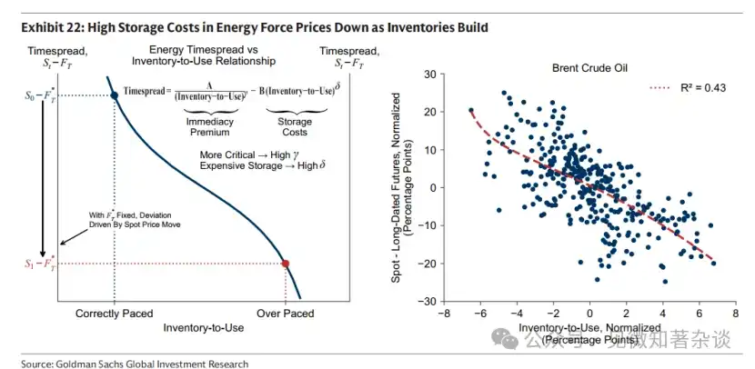
Chart 22: High storage costs in the energy sector force prices down when inventory accumulates.
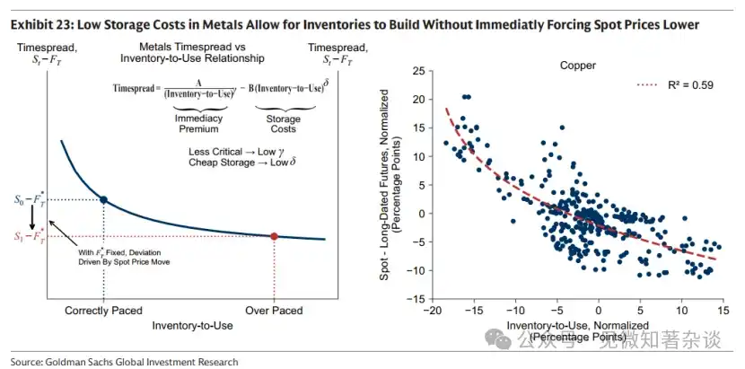
Chart 23: Low storage costs in the metals sector allow inventory to accumulate without immediately forcing spot prices down.