


On the Las Vegas Strip, slot machines have an average payout rate of about 93%, meaning you get back only $0.93 for every $1 wagered; on Polymarket, however, traders voluntarily accept payouts as low as $0.43, betting $1 on obscure outcomes with odds even worse than those in a casino.
This is not a metaphor—it’s based on real data. Researcher Jonathan Becker analyzed all settled markets on Kalshi, covering 72.1 million trades and a total trading volume of $18.26 billion. The patterns he discovered apply equally to Polymarket—the same mechanisms, the same biases, and therefore the same opportunities. The data leads to a straightforward conclusion: approximately 87% of prediction market wallets end up losing money, but the remaining 13% don’t win by luck—they employ a mathematical approach that most traders have never even heard of.
This article breaks down five game theory formulas that distinguish winners from losers, each accompanied by the corresponding mathematical principles, real-world examples, and executable Python code—traders who have already applied these methods in practice include:
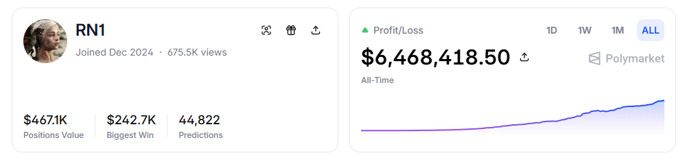
- RN (Polymarket profile: https://polymarket.com/profile/%40rn1): A Polymarket algorithmic trading bot that generated over $6 million in total profit across sports markets based on the model described in the article.
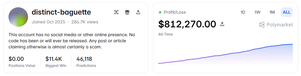
- distinct-baguette (Polymarket profile: https://polymarket.com/profile/%40distinct-baguette): Grew $560 to $812,000 by market-making on UP/DOWN markets.
I. Expected Value: The Most Fundamental Formula
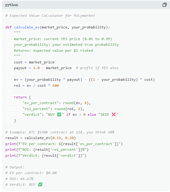
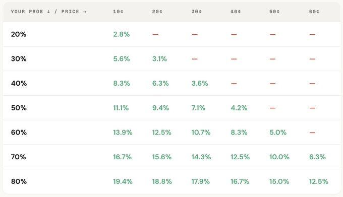
On Polymarket, every trade is essentially a calculation of expected value. Most traders rely on intuition, but the top 13% of winners make decisions using math. Expected value (EV) measures not the outcome of a single event, but the average return over many repetitions, helping you determine whether a trade is worth taking.
Using a real market as an example, “Will Bitcoin reach $150,000 before June 2026?” the current YES price is 12¢, implying a market probability of 12%. If, based on on-chain data, halving cycles, and ETF fund flows, the true probability is estimated at approximately 20%, then this trade has a positive expected value. Calculating this, each contract bought at 12¢ yields an average long-term profit of 8¢; purchasing 100 contracts costs $12 and yields an expected profit of $8, for a return rate of approximately +66.7%.
However, data shows that most prediction market traders do not perform such calculations. In a sample covering 72 million trades, takers (market buyers) lost an average of about 1.12% per trade, while makers (limit order providers) gained an average of about 1.12% per trade. The difference between them is not in information, but in patience—makers wait for positive expected value opportunities, while takers are more prone to impulsive trading.
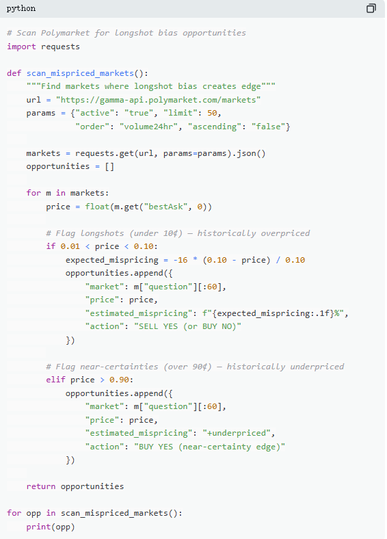
II. Mispricing: The Low-Cost Contract Trap
“Underdog bias” is one of the most expensive mistakes in prediction markets, as traders systematically overestimate low-probability events, paying too much for seemingly cheap contracts. A contract priced at 5¢ theoretically implies a 5% win probability, but on Kalshi, the actual win rate is only 4.18%, corresponding to a pricing bias of -16.36%; in more extreme cases, a 1¢ contract should imply a 1% win rate, yet for takers, the actual win rate is just 0.43%, with a bias as high as -57%.
Overall, the market prices are relatively accurate in the middle range (30¢–70¢), but significant deviations occur at the extremes: contracts priced below 20¢ tend to have actual win rates lower than the implied probability, while contracts priced above 80¢ often have higher win rates than their price suggests.
In other words, market inefficiencies are primarily concentrated at the extremes, which are precisely the areas where emotional trading is most prevalent. Specifically, there are two formulas:
Formula 1: Mispricing (δ)
Mispricing measures the deviation between the actual win rate of a contract and its implied probability. For example, with a 5¢ contract, assume there are 100,000 trades settled at 5¢ across all markets, and 4,180 of them ultimately result in YES. The actual win rate is 4.18%, while the implied probability corresponding to the price is 5.00%. The difference between the two is -0.82 percentage points, representing a relative deviation of approximately -16.36%. This means that purchasing each 5¢ contract effectively entails paying a premium of about 16.36%.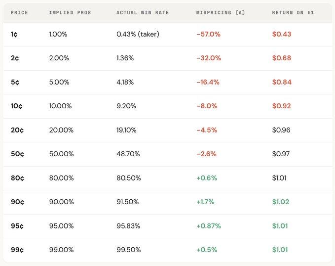
Formula 2: Single-trade excess return (Gross Excess Return, rᵢ)
If mispricing reflects a general bias, then individual excess returns reveal the actual return structure of each trade—this is where behavioral biases become clearly visible. When purchasing a 5¢ contract, two outcomes are possible: if the contract hits, the return can reach +1900% (approximately 20x return); if it misses, the loss is 100%, and the entire 5¢ investment is lost.
This is precisely why obscure preferences are appealing: when they hit, the returns are extremely high, making them easy to remember, amplify, and spread. However, overall, their actual hit rate is lower than the probability implied by the price, and the asymmetric structure between “total loss” and “extremely high reward” creates a negative expected value over many trades—essentially equivalent to buying an overpriced lottery ticket.
Overall, this bias exhibits a clear price gradient: the lower the contract price, the worse the return. For example, as a taker, for every dollar invested in a 1¢ contract, you on average recover only about $0.43; whereas for every dollar invested in a 90¢ contract, you on average receive about $1.02. The cheaper the price, the less favorable the actual trading conditions.
Further breaking down the roles reveals that this structure is nearly a mirror image: the taker’s losses in the lower price range (as low as -57%) directly correspond to the maker’s gains in the same range; the overall market pricing discrepancy lies between the two. In other words, almost every penny lost by the taker is gained by the maker.
From a game theory perspective, low-probability contracts are often systematically overvalued, while high-probability contracts are frequently undervalued. The true strategy is not to chase long shots, but to sell low-probability contracts and buy high-conviction ones.
Three: The Kelly Criterion: How Much to Bet
When a trade with positive expected value is identified, the real challenge has only just begun: how much should the trader bet? Too large a position, and a single loss could wipe out weeks of gains; too small a position, and even with an edge, growth becomes so slow as to be virtually meaningless. Between betting everything and betting nothing lies a mathematically optimal betting percentage—this is the Kelly Criterion.
The Kelly Criterion, introduced by John Kelly Jr. in 1956, was originally developed to optimize communication signal noise issues and has since been proven to be one of the most effective position sizing methods for gambling, trading, and market prediction. Professional poker players, sports betting experts, and Wall Street quantitative funds almost all use some form of the Kelly strategy.

In prediction markets, where contracts are binary (paying $1 or $0) and the price itself represents probability, the application of the Kelly criterion is more straightforward. The key is understanding the odds (b): if you buy a YES contract at 30¢, you are risking $0.30 to win $0.70, giving odds of 0.70 / 0.30 ≈ 2.33; at 50¢, the odds are 1; at 10¢, they are 9; and at 80¢, they are only 0.25. The higher the odds, the greater the Kelly criterion’s recommended bet size, assuming you have an edge.
But a key principle is to avoid using full Kelly. Although the full Kelly criterion mathematically maximizes long-term capital growth, its real-world execution involves extreme volatility, with drawdowns often exceeding 50%. While it may yield the highest returns over the long term, the intense fluctuations along the way often make it difficult for most people to stick with it. Therefore, a more common approach is to use fractional Kelly (such as 1/2 or 1/4 Kelly). For example, under stable win-rate conditions, full Kelly produces the highest final capital curve but with high volatility; 1/4 Kelly offers smoother growth and manageable drawdowns; and 1/2 Kelly strikes a balance between the two.
At its core, the Kelly Criterion provides a discipline: first determine whether an edge exists (i.e., your subjective probability exceeds the market-implied probability), and only then decide how much capital to allocate. Trading truly transitions from gambling to strategy only when both “whether to bet” and “how much to bet” are mathematically constrained.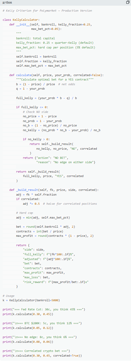
Four: Bayesian Updating: Change Your Mind Like an Expert
Predictive markets fluctuate because new information continuously enters the system. What matters is not whether the initial judgment was correct, but how you adjust your beliefs when the evidence changes. Most traders either ignore new information or overreact to it, while Bayesian updating provides a mathematical method for determining how much to adjust.
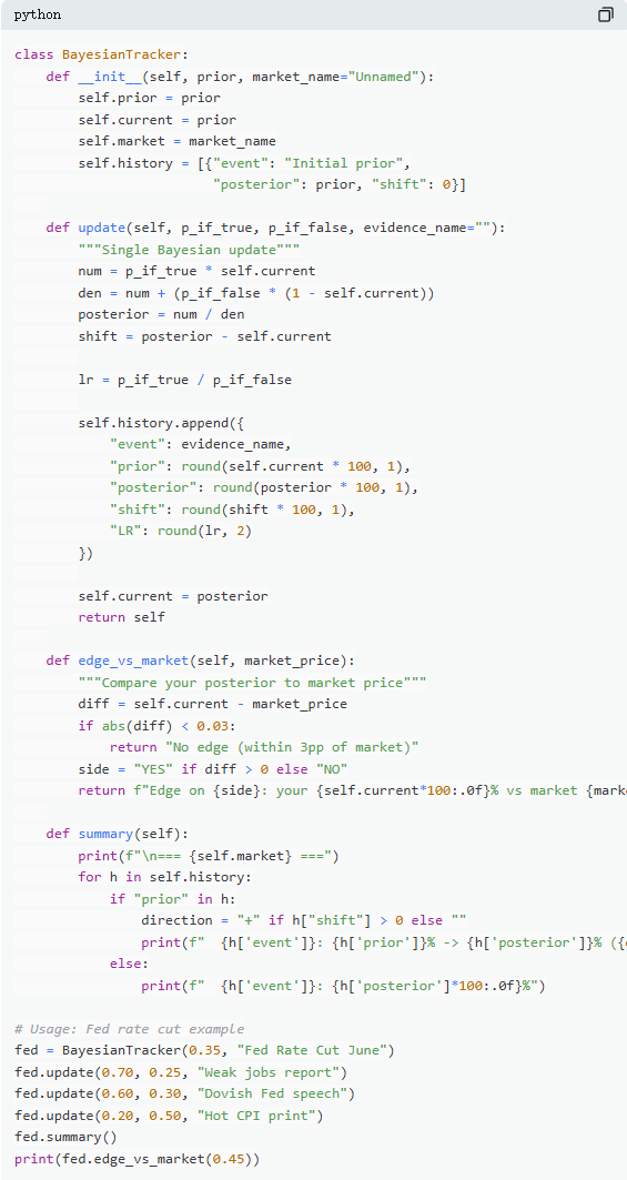
Its core logic can be simply understood as: new judgment = degree to which the evidence supports the original hypothesis × original judgment ÷ overall probability of the evidence occurring. In practice, this is typically expanded using the law of total probability to yield a more computationally convenient form.
Using a typical market as an example, “Will the Federal Reserve cut rates at its June meeting?” The current market price is 35¢, corresponding to a 35% probability, serving as the initial assessment. Subsequently, non-farm payroll data is released, showing only 120,000 new jobs (expected: 200,000), rising unemployment, and slowing wage growth. In this scenario, if the Fed does cut rates, the probability of such weak employment data occurring is relatively high, estimated at 70%; if it does not cut rates, the probability of such data occurring is lower, but still possible, estimated at 25%.
After applying Bayesian updating, the new probability is approximately 60.1%, an increase of about 25 percentage points from 35%. This means that a single key piece of information is sufficient to significantly alter market sentiment.
In practice, it is not necessary to fully calculate the formula each time. A more commonly used approach is the "likelihood ratio." The same piece of information (e.g., LR = 3) has different impacts depending on the initial assessment: starting from 10%, it may increase to about 25%; from 50%, it can rise to 75%; and from 90%, it only increases to approximately 96%. The higher the initial uncertainty, the greater the impact of the information.
The traders who consistently outperform prediction markets over the long term are not necessarily those who make the most accurate judgments, but those who can adjust their judgments the fastest and most rationally when new evidence emerges. The Bayesian approach essentially provides a measure of this “speed of adjustment.”
Five: Nash Equilibrium — The "Poker Formula" for Predicting Markets
In poker, bluffing is never a gut feeling—it’s a precisely calculable strategy. There exists an optimal bluffing frequency; deviating from it allows skilled opponents to exploit you. The same logic applies to predicting markets. On Polymarket, “bluffing” corresponds to contrarian trading—taking a position against the majority when market pricing is skewed; while “folding” is akin to passively acting as a taker, continuously paying a premium for market sentiment.
On Polymarket, makers and takers form a similar adversarial relationship. Trading against the market consensus is akin to "bluffing," while trading with the consensus is similar to "betting on value." From an equilibrium perspective, the market should render marginal participants indifferent between being a maker or a taker—a state corresponding to the Nash equilibrium in prediction markets.
However, this equilibrium is not fixed but dynamically adjusts based on changes in participant structure. Data shows that different market categories correspond to different optimal strategies: in areas with more rational information and more efficient pricing—such as financial markets—the scope for contrarian trading is smaller; whereas in areas with stronger sentiment and greater irrationality—such as entertainment and sports—the market is more prone to pricing discrepancies, creating opportunities for contrarian trading.
More importantly, this equilibrium has also changed significantly over time. In the early period (2021–2023), takers were the profitable group, and the optimal strategy favored aggressive execution; after the surge in trading volume in Q4 2024, professional market makers entered en masse, altering the market structure and shifting the equilibrium strategy toward makers (approximately 65%–70%). This is a classic outcome of game theory: when the participant structure changes, the optimal strategy evolves accordingly. Strategies that worked well in a “novice environment” can quickly become ineffective against “professional opponents,” causing the market’s “playstyle” to continuously iterate.
Summary
87% of prediction market wallets end up losing money, not because the market is manipulated, but because these traders never truly did the math. They buy obscure contracts at worse prices than slot machines, rely on gut feelings to determine position sizes, ignore new information, and pay for “optimism” with every market order.
The 13% of participants who consistently profit are not just luckier—they use these five formulas as an integrated system, creating a complete process from analysis to execution, with every step grounded in 72.1 million real trading transactions.
This window will not last forever. As professional market makers enter, the market spread is being rapidly compressed; takers had an approximate +2.0% advantage in 2022, but it has now turned to -1.12%.
The question is simply whether to evolve with the market or keep buying a $1 lottery ticket with a $0.43 return.